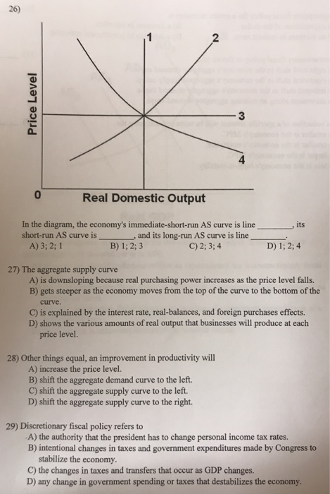
40 in the diagram, the economy's short-run as curve is line ___ and its long-run as curve is line ___.

Phillips Curve: Inflation and Unemployment. In economics, inflation refers to the sustained increase in the general price level of goods and services in an economy. Unemployment takes place when people have no jobs but they are willing to work at the existing wage rates.. Inflation and unemployment are key economic issues of a business cycle. Both are key economic … The aggregate supply curve (short-run): A) graphs as a horizontal line. B) is steeper above the full-employment output than below it. C) slopes downward and to the right. D) presumes that changes in wages and other resource prices match changes in the price level.

3 The curve JK in the diagram is a consumer's initial budget line. G ... 13 The diagram shows the cost and revenue curves of a monopolistically competitive firm in long-run equilibrium. cost, revenue O output ... 22 What will be most likely to decrease a country's national output in the short-run but to increase its potential for long-run ...

In the diagram, the economy's short-run as curve is line ___ and its long-run as curve is line ___.

In the short run, capital is fixed, firms can employ more labour (e.g. overtime) to respond to short-run increases in demand. In the short run, we typically draw the curve as a straight line. However, in practice, the SRAS could become more inelastic as a firm gets closer to full capacity. Long-run aggregate supply curve. There are two main ... 1 In the diagram, a firm is operating at point X on its long-run average cost curve. cost output O X Q LRAC Which statement is not correct? A The firm is employing the least-cost combination of factor inputs to produce OQ. B The firm is operating below its minimum efficient scale. C The firm is producing at its cost-minimising level of output. Answer Option 4 The short-run AS curve is upward slopi …. View the full answer. Transcribed image text: In the diagram, the economy's short-run AS curve is line , and its long-run AS curve is line is 3:4. Previous question Next question.

In the diagram, the economy's short-run as curve is line ___ and its long-run as curve is line ___.. A a reduction in the economy's long-run production possibility ... D an increase in the number of adults experiencing the economic problem 2 What is likely to be the short-run consequence of replacing central planning with a market-based ... 7 In the diagram D1D1 is a straight line demand curve and D2D2 is a rectangular hyperbola curve. M N ... An economy's aggregate demand curve shifts leftward or rightward by more than changes in initial spending because of the D. multiplier effect In the above diagram, the economy's immediate-short-run aggregate supply curve is shown by line: In the above diagram, the economy's long-run aggregate supply curve is shown by line: A) 1. B) 2. C) 3. D) 4. A. In the above diagram, the economy's relevant aggregate demand and long-run aggregate supply curves are lines: A) 4 and 2. B) 4 and 1. C) 2 and 4. D) 2 and 3. B. In the above diagram, the economy's short-run AS curve is line ___ and ... The Long-Run Curve. The Long-Run Aggregate Supply (LRAS) curve is completely vertical. You're probably asking why. It's because the real GDP in the long-run is dependent on the supply of capital, labor, raw materials, and other factors outside of price.

The procedure of deriving the long run industry supply curve is different since, in the long run, entry into and exit of firms from the industry come into action. A competitive firm in the long run produces at that point where the long run MC curve intersects the long run AC curve at the lowest point (i.e., P = AR = MR = LMC = minimum point of ... Mar 15, 2019 · In the diagram the economys short run as curve is. Aggregate supply has decreased equilibrium output has decreased. In the diagram the economys immediate short run as curve is line its short run as curve. At point p the long run marginal cost curve intersects the long run average cost. 34 refer to the above diagram. The economic relationship the short run average total cost (SRATC) and the long run average total cost (LRATC) is pretty straight forward if you understand these other concepts: The short run average total cost curve has the U shape because of diminishing marginal product. Diminishing marginal product means that there are diminishing returns from the variable input in the short run. All figures are in billions. if the economy was closed to international trade, the equilibrium GDP and the multiplier would be. $350 and 5. If Carol's disposable income increases from $1,200 to $1,700 and her level of saving increases from minus $100 to a plus $100, her marginal propensity to: consume is three-fifths.

In the diagram, the economy's long-run aggregate supply curve is shown by line: 1. Answer the question on the basis of the following table for a particular country in which C is consumption expenditures, Ig is gross investment expenditures, G is government expenditures, X is exports, and M is imports. Oct 13, 2019 · In the diagram the economys immediate short run as curve is line its short run as curve. Refer to the diagrams in which ad 1 and as 1 are the before curves and ad 2 and as 2 are the after curves. In the diagram the economys short run as curve is. The long run is a period of time which the firm can vary all its inputs. The diagram above portrays the short and long run equilibrium. The point where aggregate demand intersects with the vertical line is what determines the level of output. In a classical economics world, if there is a shock to aggregate demand, the price level adjusts to return the economy to its natural level of output and return employment to ... Transcribed image text: 26) 2 3 C3 4 0 Real Domestic Output In the diagram, the economy's immediate-short-run AS curve is line short-run AS curve is , and its long-run AS curve is line C) 2:3;4 A) 3; 2;1 B) 1; 2;3 D) 1:2,4 27) The aggregate supply curve A) is downsloping because real purchasing power increases as the price level falls. B) gets ...

7. In the long run, a firm can adjust the factors of production that are fixed in the short run; for example, it can increase the size of its factory. As a result, the long-run average-total-cost curve has a much flatter U-shape than the short-run average-total-cost curve.

Relationship of the Short-Run Average Cost Curves and the Long-Run Average Cost Curve LAC: In the short run, some inputs are fixed and others are varied to increase the level of output. The long run is a period of time which the firm can vary all its inputs. In long run none of the factors is fixed and all can be varied to expand output.

Understanding Short-Run and Long-Run Average Cost Curves The long-run average cost (LRAC) curve is a U-shaped curve that shows all possible output levels plotted against the average cost for each level. The LRAC is an "envelope" that contains all possible short-run average total cost (ATC) curves for the firm. It is made up of all ATC curve tangency points.

In the same way, if the firm's output is to be q 3 on IQ 3 (q 3 > q 2), then the firm would be in equilibrium at the point E 3 (x 3, y).. If we now join the points E 1, E 2, E 3, etc. by a curve, we would get the short-run expansion path of the firm in the one variable and one fixed input case.This expansion path would be a horizontal straight line like GH in Fig. 8.15, since y is constant ...

11.3 Short-run and long-run equilibria 11.4 Prices, rent-seeking, and market dynamics at work: Oil prices 11.5 The value of an asset: Basics 11.6 Changing supply and demand for financial assets 11.7 Asset market bubbles 11.8 Modelling bubbles and crashes

IS LM Model Questions and Answers. Get help with your IS–LM model homework. Access the answers to hundreds of IS–LM model questions that are …

14 The aggregate supply curve (short-run): A. graphs as a horizontal line. B. is steeper above the full-employment output than below it. C. slopes downward and to the right. D. presumes that changes in wages and other resource prices match changes in the price level. 15 The aggregate supply curve (short-run) is upsloping because:

3 The curve GH in the diagram is a consumer's initial budget line. G J HK good Y ... 9 The diagram shows a firm's short-run and long-run average cost curves. O output ... Which curve could show the economy's new consumption function following a reduction in the

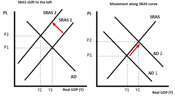
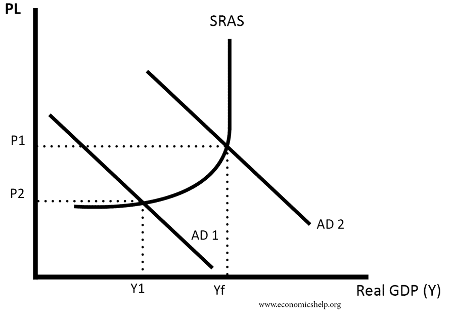
The short-run aggregate supply curve increased as nominal wages fell. In this analysis, and in subsequent applications in this chapter of the model of aggregate demand and aggregate supply to macroeconomic events, we are ignoring shifts in the long-run aggregate supply curve in order to simplify the diagram.

Short-run aggregate supply (SRAS) — During the short-run, firms possess one fixed factor of production (usually capital), and some factor input prices are sticky. The quantity of aggregate output supplied is highly sensitive to the price level, as seen in the flat region of the curve in the above diagram.

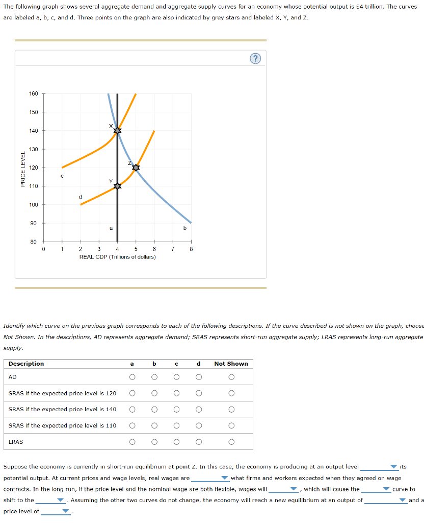
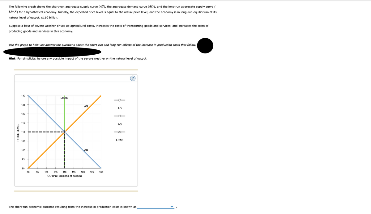
The graph to the right shows aggregate demand, long-run aggregate supply, and the short-run aggregate supply curve. The economy is in short-run equilibrium at E1. 1. The current situation would be described as _____.

Short-run and Long-run Supply Curves (Explained With Diagram) In the Fig. 24.1, we have given the supply curve of an individual seller or a firm. But the market price is not determined by the supply of an individual seller. Rather, it is determined by the aggregate supply, i.e., the supply offered by all the sellers (or firms) put together.

The relationship between long-run and short-run aggregate supply is that the LRAS curve is a result of a combination of many SRAS curves. The short-run aggregate is prone to frequent changes by ...

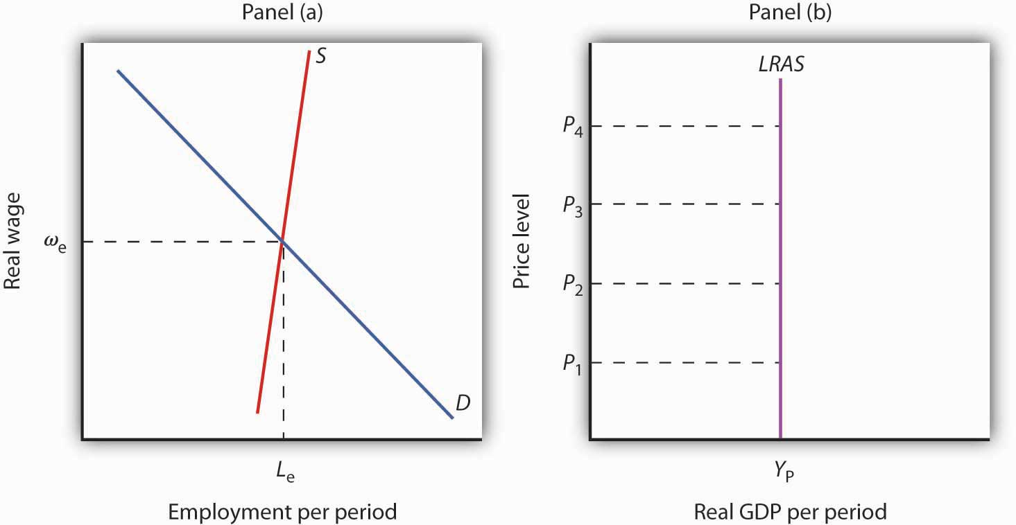
Long-Run Aggregate Supply. The long-run aggregate supply (LRAS) curve relates the level of output produced by firms to the price level in the long run. In Panel (b) of Figure 22.5 "Natural Employment and Long-Run Aggregate Supply", the long-run aggregate supply curve is a vertical line at the economy's potential level of output.There is a single real wage at which employment reaches its ...

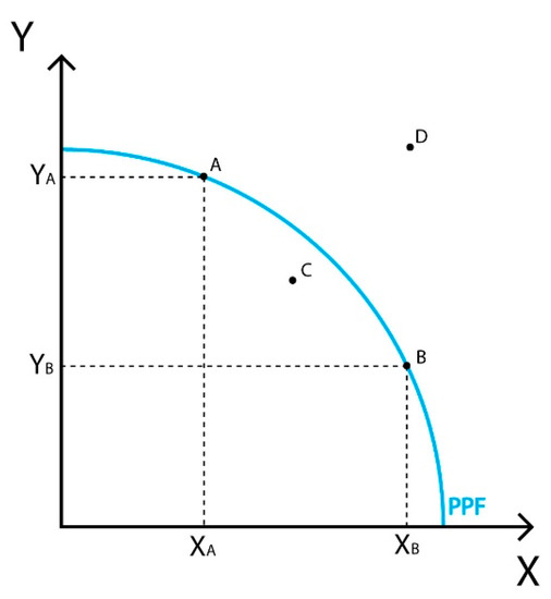
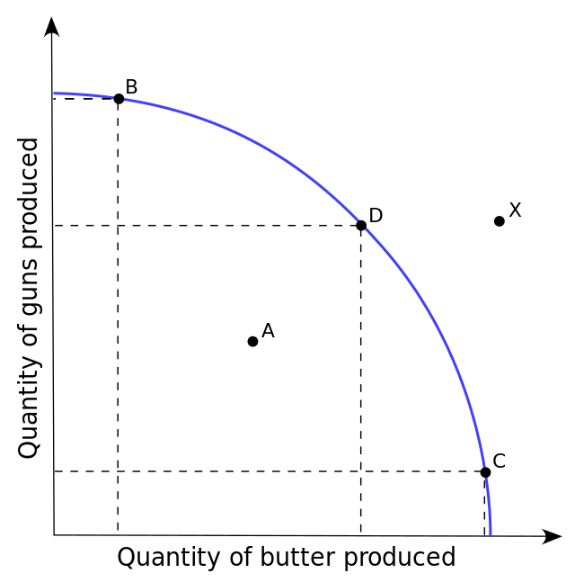
Production-Possibility Frontier delineates the maximum amount/quantities of outputs (goods/services) an economy can achieve, given fixed resources (factors of production) and fixed technological progress.Points that lie either on or below the production possibilities frontier/curve are possible/attainable: the quantities can be produced with currently available resources and …

The relationship between short run and long run cost curves is explained in the following diagram: In the diagram, output is shown along OX axis. Costs are shown along OY oxis, SACS1, ; SAC2 and SAC3 are the three short run average cost curves of three different plants and machinery. SAC denotes the short run costs of plant 'A'.

In the long run, the Phillips curve is a vertical line at the natural rate of unemployment. ADVERTISEMENTS: This natural or equilibrium unemployment rate is not fixed for all times. Rather, it is determined by a number of structural characteristics of the labour and commodity markets within the economy.

The new-Classical explanation - the importance of expectations. Although there are disagreements between new-Classical economists and monetarists, the general line of argument about the breakdown of the Phillips curve runs as follows. Assume that the economy starts from an equilibrium position at point A, with inflation currently at zero, and unemployment at the natural rate of 10% (NRU = 10%).

Get help with your Production–possibility frontier homework. Access the answers to hundreds of Production–possibility frontier questions that are explained in a way that's easy for you to ...

3 The line RS in the diagram is a consumer's budget line. O R S quantity of X M N quantity ... 23 What is likely to decrease a country's actual output in the short run but may increase its long-run ... 26 In the diagram, the curve X 1 shows an economy's initial trade-off between inflation and unemployment. X1 X2

In Fig. 4.6 we have drawn the long run Phillips curve as a vertical line through the 'natural rate of unemployment'. Further, we have drawn three short run Phillips curves (SRPC 1 , SRPC 2 and SRPC 3 ) representing different expected rates of inflation.

Start studying EC. ch 12. Learn vocabulary, terms, and more with flashcards, games, and other study tools.

Answer Option 4 The short-run AS curve is upward slopi …. View the full answer. Transcribed image text: In the diagram, the economy's short-run AS curve is line , and its long-run AS curve is line is 3:4. Previous question Next question.

1 In the diagram, a firm is operating at point X on its long-run average cost curve. cost output O X Q LRAC Which statement is not correct? A The firm is employing the least-cost combination of factor inputs to produce OQ. B The firm is operating below its minimum efficient scale. C The firm is producing at its cost-minimising level of output.